Chilling requirements : {{chilling_target}} units
Forcing requirements : {{forcing_target}} °C.{{unit}}
Welcome to the PhenoWeather Serious Game!
This serious game has been developed to explore the impacts of climate change on grapevines and apples. It is based on weather simulations coupled with phenological and yield models for different climate scenarios, geographic locations and plant varieties.
Understanding the Science
Learn about the science behind the game
The
Climate
tab explains weather models, climate scenarios (RCP), and data sources that drive the simulations.
The
Phenology & Yield
tab describes the biological models for grapevines and apples, climate change impacts, and how yield is estimated using the Hester model.
Explore the Data
Visualize and analyze
The
Maps
tab provides spatial visualization of sites and scenarios.
The
Outputs
tab shows simulated budburst, bloom, and harvest dates.
The
Risks
tab calculates probabilities of frost, heat stress, and other climate risks.
The
Catalog
tab shows the catalog of varieties.
• The climate scenarios (RCP) used in the game modes are not perfect and might have some bias and smooth extremes; the Stochastic Weather Generator (SWG) used to generate weather simulations also has limitations (see associated Climate tab).
• The phenological and yield models have been trained with limited data for each variety and might not be well adapted for some locations/species (see associated Phenology tab).
• Finally, the economy of the game might not yet be very realistic (feedback welcome).
Game Mode
Test your adaptation strategies in an interactive game! Establish your agricultural estate with a budget of 300,000 € and manage it over 60 years (2026-2086). Buy plots of grapevines or apples, invest in risk-mitigation infrastructures, and advance through decades to see the impacts of climate change on your yields and finances. Can you sustain a positive budget until the next century?
Credits
Latitude
{{ station.lat }}
Longitude
{{ station.lon }}
| Days | Sim 1 (%) | Sim 2 (%) |
|---|---|---|
| {{t[0]}} | {{t[1]}} | {{t[2]}} |
| Consecutive days | Sim 1 (%) | Sim 2 (%) |
|---|---|---|
| {{t[0]}} | {{t[1]}} | {{t[2]}} |
Spring frost is one of the most damaging climate hazards for perennial crops. Once budburst occurs, young shoots, leaves, and flower buds become highly vulnerable to freezing temperatures. Frost damage causes cell membrane rupture, tissue necrosis, and can lead to complete crop loss if it occurs during flowering.
Critical thresholds: Damage begins around -2°C for young buds and intensifies below -4°C. The risk window extends from budburst through flowering (typically March–May in temperate regions).
For each weather simulation i and year y:
- Identify the budburst date BB i,y using the phenology model
- Count days with T min below the threshold (default: -2°C) between budburst and June 1st
- Compute probability distributions: P(N frost days) = k/n, where k is the count with N frost days and n is the total simulations
The consecutive frost days metric identifies the maximum length of uninterrupted cold spells, particularly damaging as it prevents plant recovery.
| Days | Sim 1 (%) | Sim 2 (%) |
|---|---|---|
| {{t[0]}} | {{t[1]}} | {{t[2]}} |
| Consecutive days | Sim 1 (%) | Sim 2 (%) |
|---|---|---|
| {{t[0]}} | {{t[1]}} | {{t[2]}} |
Extreme heat affects plant physiology through multiple pathways: photosynthetic inhibition, enzyme denaturation, accelerated fruit maturation, and reduced sugar-acid balance. For grapevines, prolonged heat exposure during ripening degrades anthocyanin accumulation and aroma compound synthesis. For apples, heat can cause sunburn, reduced fruit size, and premature drop.
Critical thresholds: Photosynthesis declines above 30°C, with severe stress occurring above 35–40°C. Grapevines are assessed using daily maximum temperature ( T max ), while apples use mean temperature ( T mean ) due to different physiological sensitivities.
For each simulation and year:
- Define the heat-sensitive period (typically flowering to harvest)
- For grapevines: count days where T max > threshold (default: 35°C)
- For apples: count days where T mean > threshold (default: 35°C)
- Calculate probabilities as in the freezing case
Consecutive heat days are particularly harmful because they compound heat stress and prevent nocturnal recovery. Heat waves (3+ consecutive days above threshold) have disproportionate impacts on yield and quality (Jones et al., 2005).
| Class | Thresholds | Sim 1 (%) | Sim 2 (%) |
|---|---|---|---|
| {{t[0]}} | {{t[1]}} | {{t[2]}} | {{t[3]}} |
Precipitation data unavailable
The De Martonne aridity index is calculated from the ratio between precipitation (P) and temperature (T).
The historical weather records selected for this site currently only contain temperature data, making aridity calculation impossible. Please select data from climate model projections to visualize this index.
Water availability is fundamental to plant growth, photosynthesis, and fruit development. Drought stress closes stomata (reducing CO₂ uptake), limits nutrient transport, and reduces canopy growth. For grapevines, moderate water stress during ripening can improve quality, but severe stress reduces yield and causes berry shrivel.
The De Martonne Aridity Index integrates precipitation and temperature to characterize water availability, accounting for evaporative demand driven by temperature.
Calculated for the growing season (typically April–September):
Where P = cumulative precipitation (mm), T = mean temperature (°C). The constant 10 prevents division by zero.
Classification: I DM < 10: Arid; 10–20: Semi-arid; 20–30: Sub-humid; ≥ 30: Humid.
| Risk intensity | Index (P × T) | Sim 1 (%) | Sim 2 (%) |
|---|---|---|---|
| {{t[0]}} | {{t[1]}} | {{t[2]}} | {{t[3]}} |
Precipitation data unavailable
The Branas hydrothermal index evaluates downy mildew risk by combining precipitation and temperature (P × T).
The selected historical records do not contain precipitation data. Try using a climate model dataset instead.
Downy mildew ( Plasmopara viticola) is a devastating grapevine pathogen requiring both warmth and moisture for infection and sporulation. It causes leaf necrosis, reduces photosynthetic capacity, and can destroy entire crops if untreated.
The Branas Hydrothermal Index combines precipitation and temperature as a proxy for disease pressure. Higher values indicate more favorable conditions for pathogen development.
Calculated for the growing season (typically April–September):
Where P i = daily precipitation (mm) and T i = daily mean temperature (°C), summed over the entire growing season.
Risk Classification: BHI < 2500: Low; 2500–5100: Moderate; 5100–7500: High; ≥ 7500: Very high risk.
No probability data available
Adjust your selections above and click the "LOAD DATA"� button for the corresponding simulation.
Geophysical Research Letters, 35(12), L12703.
https://doi.org/10.1029/2008GL033955
Demonstrates that earlier budburst driven by warming paradoxically increases frost exposure risk.
Climatic Change, 73(3), 319–343.
https://doi.org/10.1007/s10584-005-4704-2
Quantifies relationships between growing-season temperatures, heat extremes, and wine quality.
Comptes Rendus de L'Acad. Sci., Paris, 3, 1395–1398.
Original formulation of the aridity index widely used in hydroclimatology and agroclimate classification.
Déhan, Montpellier.
Seminal viticulture reference defining hydrothermal indices for disease risk assessment.
Biology Letters, 8(5), 795–798.
https://doi.org/10.1098/rsbl.2012.0226
Reviews how climate change alters pathogen pressure, including downy mildew risk under future scenarios.
Contribution of Working Group II to the Sixth Assessment Report of the IPCC.
https://www.ipcc.ch/report/ar6/wg2/
Comprehensive assessment of climate risks to agriculture, including heat stress, water scarcity, and shifting disease patterns.
Explore this catalog to compare the agronomic traits and financial metrics of each variety before making your planting decisions.
Some notion about climate, models and data useful to understand agricultural impacts.
Physics-based models (also called General Circulation Models or GCMs) represent all known physical processes of the Earth system: atmospheric dynamics, ocean circulation, land surface, ice sheets, etc. They are linked to Regional Climate Models (RCMs) for higher-resolution in specific regions.

Stochastic Weather Generators (SWGs) are statistical models that learn the probability distributions of weather variables (temperature, precipitation...) from observed or simulated data, then generate large ensembles of synthetic daily time series.

To project future climate, scientists define Representative Concentration Pathways (RCPs) — standardised scenarios describing how greenhouse gas concentrations in the atmosphere could evolve depending on human choices and policies.
Simulation with the climate models on the historical period. It is used as a baseline for comparison.
Strong mitigation. Global warming limited to ~+1.5–2°C by 2100. Requires drastic emission cuts starting now.
Moderate mitigation. Warming of ~+2–3°C by 2100. Policies reduce but don't eliminate emissions.
“Business as usual”. Warming of ~+4–5°C by 2100. No significant climate policy is implemented.
Three main data sources are used in climate studies
Direct measurements at specific locations. The most reliable data source — what is actually observed in the field.
Reanalyses blend observations from stations, satellites and radiosondes with a climate model to reconstruct a spatially complete historical climate.
Future climate projections derived from physics-based climate models under different RCP forcing trajectories. They extend beyond the observation period into the future.
Understanding how apple trees and grapevines move through their annual growth cycle — and why climate change matters.
Phenology is the study of cyclic and seasonal biological events and their relationship with climate and environment. For fruit trees such as apples and grapevines, the key annual stages are:
Phenological models are built around two sequential accumulation processes:
Cold temperatures accumulate as chilling units during autumn and winter. Once a chilling requirement is met, endo-dormancy is broken.
Warm temperatures accumulate as growing degree days (GDD, above a base temperature). Once a forcing requirement is met, budburst occurs.

The figures below place the dormancy and budburst stages described above within the complete yearly cycle of the apple tree and grapevine. Three broad phases can be distinguished:
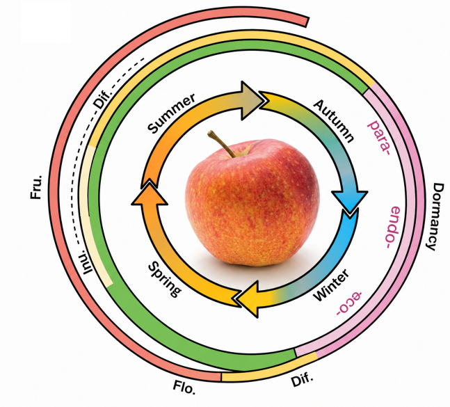
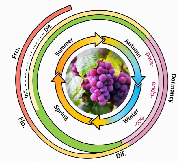
Climate change affects phenology through two interacting mechanisms: warmer winters reduce chilling accumulation while warmer springs accelerate forcing. The net effect is complex and variety-dependent.
In addition to predicting phenological dates, this game estimates yield using the Hester model (Hester & Cacho, 1997, 2003). This model calculates daily carbon balance of fruit trees based on daily temperature and phenological dates (budburst and flowering).
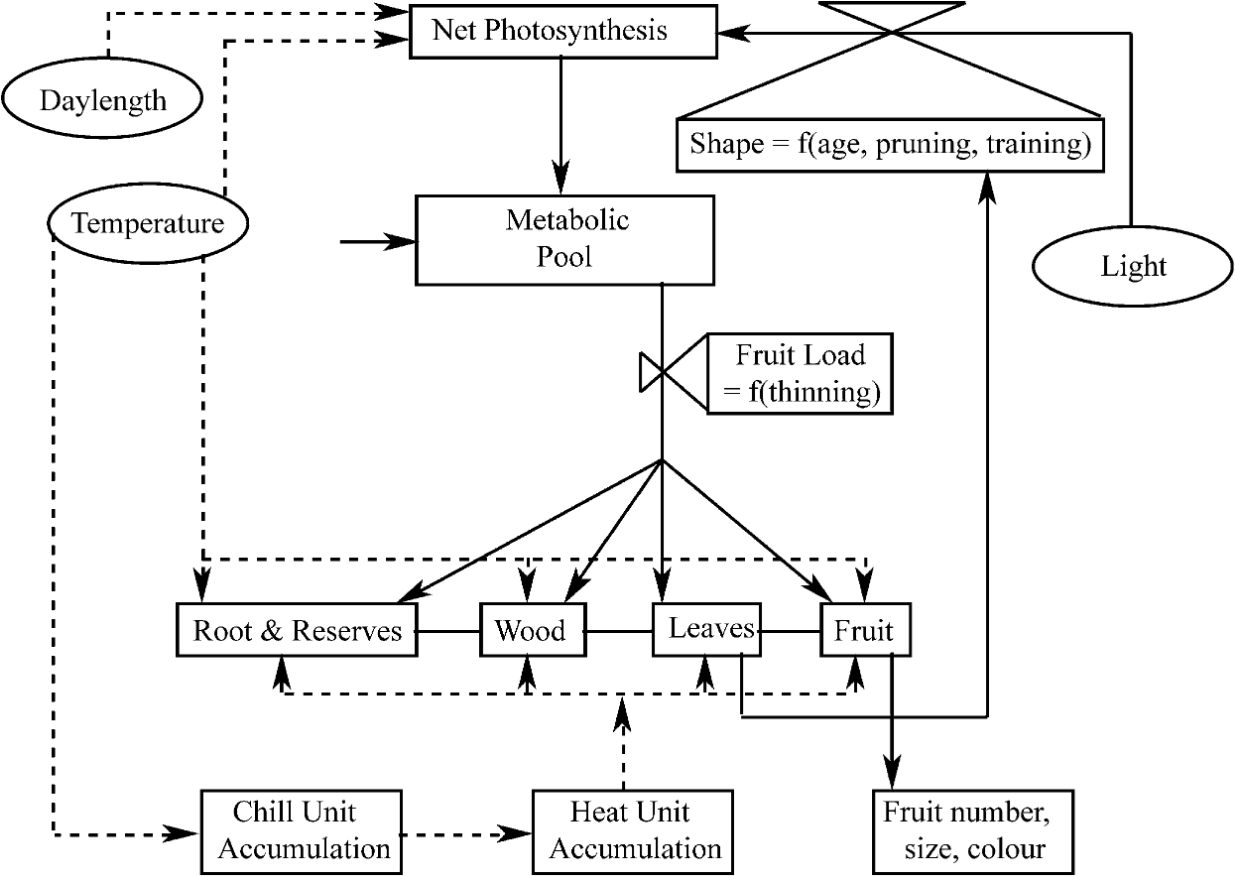
A Stochastic Weather Generator trained on historical or projected climate data produces one or multiple synthetic daily temperature sequences for the selected site and scenario.
Each synthetic sequence is fed to the phenological model for the selected species and variety. Chilling and forcing units are accumulated day by day until the respective thresholds are met.
The resulting distribution of budburst and bloom dates gives probabilities and uncertainty intervalsfor each year — including rare events like chilling failure or extreme late frosts. The Risk panel computes the probability of frost, heatwaves, and drought during sensitive periods, which can further reduce yield.
The Hester model uses daily temperatures and phenological dates to estimate yield via carbon balance calculations, adjusted by risk indices from the Risk panel.
The following references provide the scientific foundation for the phenological models and climate change impacts described in this section.
Welcome to your new agricultural domain. You have an initial budget of 300,000 € to establish your estate.
- Buy plots of grapevines or apples tailored to your strategy.
- Invest in infrastructures to mitigate climate risks (frost, heat, drought, disease).
- Advance decade by decade and analyze the agronomic and financial impacts.
Protects the market value of your apples in case of ultra-early harvest caused by heat waves, by allowing temporary off-market storage.
Unlocks terroir expansion. Allows you to acquire and operate new plots in secondary locations with different climate profiles.
Review historical performance, track phenological shifts, and understand the agronomic impact of climate extremes on your plots.
| Plot | Geographical Site | Area | Net Income (€) |
|---|---|---|---|
|
|
{{ plot.site }} | {{ plot.area_ha }} ha | {{ (plot.last_net_revenue || 0).toLocaleString('fr-FR', { style: 'currency', currency: 'EUR', maximumFractionDigits: 0 }) }} |
- Average yield: {{ (log.avg_yield * 100).toFixed(0) }} %
- Net revenue: {{ log.net_revenue.toLocaleString('fr-FR', {style: 'currency', currency: 'EUR', maximumFractionDigits: 0}) }}
- {{ signal }}
Understand how climate risks are assessed, how protections interact with varietal genetics, and the economic logic that drives your estate.
The climate engine of this game is driven by real physics. The chain of cause and effect is direct:
CO₂ & GHG emissions
Fossil fuels, land use, deforestation
Greenhouse effect ↑
Mean temperature rise
+1.5°C to +4°C by 2100
This warming is not uniform: it shifts the timing of frost windows, accelerates phenological stages, intensifies summer heat, and alters precipitation patterns — all of which directly impact your crops.
No significant mitigation of emissions. Average global temperatures rise by +3.7°C to +4.8°C by 2100. This is the most agronomically challenging scenario, and the one used to generate the climate projections in this game. It represents what happens if the world continues on its current emissions trajectory.
The climate data comes from bias-corrected regional model outputs (DRIAS portal). Decade-to-decade variability is stochastic — even under RCP 8.5, some decades will be cooler or wetter than average.
The lifecycle of both grapevines and apple trees is governed by temperature, but the two crops differ significantly in their thermal requirements and the models used to predict their key development dates.
Both crops accumulate heat daily once temperature exceeds a base threshold T base. Each day's contribution is:
These daily values accumulate from a reference date. The crop reaches each phenological stage (budburst, bloom, harvest) when cumulative GDD crosses a genetically defined threshold.
| Parameter | 🍇 Grapevine | 🍎 Apple |
|---|---|---|
| Base temperature (T base) | 10°C | 6°C |
| Chilling requirement | Low – moderate | High (critical) |
| Phenology model | BRIN (Bidabe / Garcia) | Sequential (Utah style) |
| Harvest GDD target | 1 150–1 400 GDD | 1 850–2 150 GDD |
| Market timing bonus | Fixed price (quality-based) | Up to +30% for early harvest |
| Irrigation allowed? | ⚠ Loses AOC label (−67% price) | ✓ Yes, no penalty |
Each risk is assessed during its specific phenological window. The base damage (before any mitigation from infrastructure or varietal resistance) depends on the severity level reached:
• Level 2 (Severe/Multiple frosts) → 80% base crop loss
• Level 2 (≥ 5 consecutive days > 35°C, or > 40°C) → 65% base crop loss
• Level 2 (Arid) → 55% base crop loss
• Level 2 (Severe epidemic) → 65% base crop loss
Once the actual loss from each risk is computed, they combine multiplicatively — not additively. The final harvest fraction retained is:
This ensures simultaneous shocks are far more destructive than sequential ones of the same magnitude. A year with three simultaneous Level 2 events without any adaptation destroys 97.5% of the harvest. With protections and resistant varieties, the same year becomes manageable.
No climate event causes its full base damage in isolation. Two independent shields reduce it multiplicatively:
Neither shield is absolute on its own — combining both is always stronger than either alone. The key insight: a resistant variety with good infrastructure can reduce 80% base frost damage to under 10%.
| Variety | Frost Resist. | Infrastructure | Efficacy | Calculation | Crop Lost | Crop Saved |
|---|---|---|---|---|---|---|
| Chardonnay | 0.0 | None | — | 80% × 1.0 × 1.0 | 80% | 20% |
| Chardonnay | 0.0 | Frost Nets (0.55) | 0.55 | 80% × 1.0 × 0.45 | 36% | 64% |
| Chardonnay | 0.0 | Heat Pads (0.70) | 0.70 | 80% × 1.0 × 0.30 | 24% | 76% |
| Riesling | 0.3 | None | — | 80% × 0.70 × 1.0 | 56% | 44% |
| Riesling | 0.3 | Heat Pads (0.70) | 0.70 | 80% × 0.70 × 0.30 | 17% | 83% |
French AOC regulations prohibit irrigation. If you install an Irrigation system on a variety marked "loses AOC if irrigated", your selling price drops to 33% of the AOC price — even if you increase yield. Economically, this is almost always a losing proposition.
Every decision on your estate has a financial dimension. Understanding the return on investment (ROI) and market mechanics is crucial to remaining solvent.
Each infrastructure has a one-time installation cost (capex) and an annual maintenance cost (opex). The strategic question is whether the crop value saved during a bad event outweighs the total 10-year cost.
| Infrastructure | Efficacy | Capex | OPEX/yr | 10-yr total | When to choose it |
|---|---|---|---|---|---|
| Frost Nets | 55% | 4 000 € | 200 € | 6 000 € | Budget option. Moderate frost risk or lower-value crops. |
| Heat Pads | 70% | 5 500 € | 1 500 € | 20 500 € | Worth it with ≥ 2 Frost L2 events per decade on a high-value variety. |
| Geoengineering | 100% | 50 000 € | 5 000 € | 100 000 € | Extreme risk only. Very hard to amortise on a single hectare. |
For apple varieties, the selling price is not fixed — it depends on how early or late your harvest date falls relative to the global seasonal average. Climate warming accelerates phenology, potentially letting you harvest before competitors.
| Harvest timing vs. average | Price modifier | Explanation |
|---|---|---|
| More than 15 days early | +30% | First fruit on the market — scarcity premium |
| 5 to 15 days early | +10% | Still ahead of most competitors |
| Within 10 days of average | Nominal | Normal market conditions |
| 10 to 20 days late | −10% | Market saturation beginning |
| More than 20 days late | −30% | Without cold storage — market window missed |
| More than 20 days late + Cold Storage | Nominal | Cold storage extends the market window |
The models, indices, and climate projections used in this game are grounded in peer-reviewed literature. Key references by topic:
de Martonne, E. (1926). Une nouvelle fonction climatologique : l'indice d'aridité. La Météorologie, 2, 449–458.
Branas, J., Bernon, G., & Levadoux, L. (1946). Éléments de viticulture générale.
Winkler, A.J., Cook, J.A., Kliewer, W.M., & Lider, L.A. (1974). General Viticulture. University of California Press, Berkeley.
Hester, S.M., & Cacho, O. (2003). Modelling apple orchard systems. Agricultural Systems, 77(2), 137–154.
The "News Bulletins" that appear during the game are inspired by reports on climate change impacts and adaptation pathways (e.g., IPCC AR6 WGII 2022, World Bank 2021). Important Disclaimer: These news events are fictionalized predictions created to enhance gameplay immersion and provide dynamic challenges. While grounded in realistic climate trend scenarios (RCP 2.6, 4.5, 8.5), they do not represent guaranteed, scientifically founded exact events for specific years.
Are you sure you want to return to the dashboard?
Your current progress will be lost.
Are you sure you want to uproot plot #{{ selected_plot_id_for_uproot }}?
This action is irreversible. A residual value of 15% of the initial planting CAPEX will be added to your treasury (wood resale, restructuring bonus).
| Plot ID | Gross Rev. | Est. OPEX | Net Income | Status |
|---|---|---|---|---|
| #{{ plot.id }} - {{ plot.variety_name }} | {{ (plot.last_gross_revenue || 0).toLocaleString('fr-FR', { style: 'currency', currency: 'EUR', maximumFractionDigits: 0 }) }} | - {{ ((plot.last_gross_revenue || 0) - (plot.last_net_revenue || 0)).toLocaleString('fr-FR', { style: 'currency', currency: 'EUR', maximumFractionDigits: 0 }) }} | {{ (plot.last_net_revenue || 0).toLocaleString('fr-FR', { style: 'currency', currency: 'EUR', maximumFractionDigits: 0 }) }} |
Yield: {{ ((plot.last_yield_multiplier || 0) * 100).toFixed(0) }}%
|
(This event can impact your agricultural yields or your budget).
You played the RCP 8.5 Scenario, the most pessimistic climate trajectory. As you may have experienced, technological adaptations (nets, irrigation, cold storage) quickly reach their limits against the accumulation of extreme events (relentless heatwaves, lack of winter chill). Adaptation alone is extremely costly and ultimately insufficient to save the farm if emissions continue at this rate.
You played in a Stabilization Scenario (RCP 2.6 or 4.5). While climate shocks are still present, strategic crop management (shifting terroirs, choosing resistant varieties) combined with targeted infrastructures allows for economic viability. Anticipation and early transition are the keys to resilience.
You played in a temperate, stabilized control scenario. While the weather is unpredictable, extremes remain manageable. But what would happen to your strategy if the global temperature increased by 4°C?